Delta 机器人的动力学建模#

Delta 机器人 是一种三自由度的常用并联型机器人. 由于其特殊设计, 能够保证其顶板始终平行于底板, 只有三个平动自由度而无转动. 这一点很容易证明, 此处不再赘述. 因此我们将按下面的模型讨论

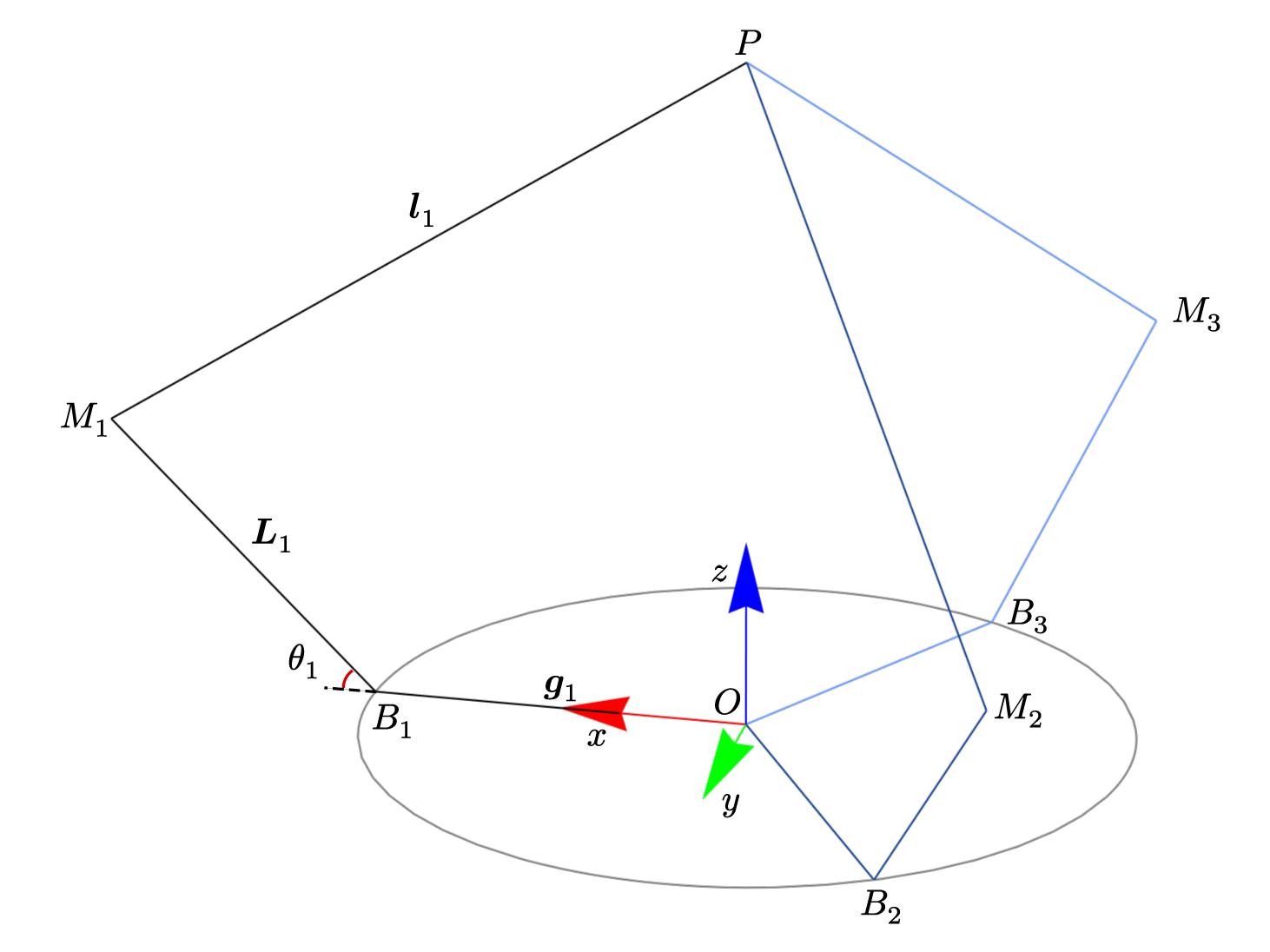
机器人有三个可以独立活动的支部, 编号为 \(1\), \(2\), \(3\), 按右手顺序排列, 彼此相隔 \(\frac{2\pi}{3}\). 我们之后的讨论将更多只限于同一个支部, 在不引起误会的情况下, 将省略下标以求简洁. 此时我们讨论的将是适用于三支的通用关系.

约定粗体 \(\mathbf{L}\) 代表向量, 非粗体的相同字母代表其模长 \(L := \|\mathbf{L}\|\). 在模型中, \(L_i\), \(i = 1,2,3\) 都是等长的, 因此都记为 \(L\); \(g\) 与 \(l\) 同理. 单位坐标轴方向为 \(\hat{\mathbf{i}}\), \(\hat{\mathbf{j}}\), \(\hat{\mathbf{k}}\); \(\hat{\cdot}\) 表示归一化. \(P\) 为关心的末端位置.

正向运动学#

正向运动学解决的问题是如何通过已知的广义坐标 \(\theta_i\), \(i = 1,2,3\) 来得到 \(P\) 的位置. 我们将从底部开始, 逐步地依次求解 \(B\), \(M\) 直到 \(P\) 的位置.

中途向量#

\(\mathbf{g}\) 与 \(B\) 的求解是极为简单的. 记方位角 \(\phi\) 为三支在水平面上的偏角, 有 \(\phi_1 = 0\), \(\phi_2 = \frac{2\pi}{3}\), \(\phi_3 = \frac{4\pi}{3}\). 于是

因为 \(M\) 始终在 \(\hat{\mathbf{k}}\) 与 \(\mathbf{g}\) 张成的平面上, 使用这两个向量作为基底来表示, 注意归一化.

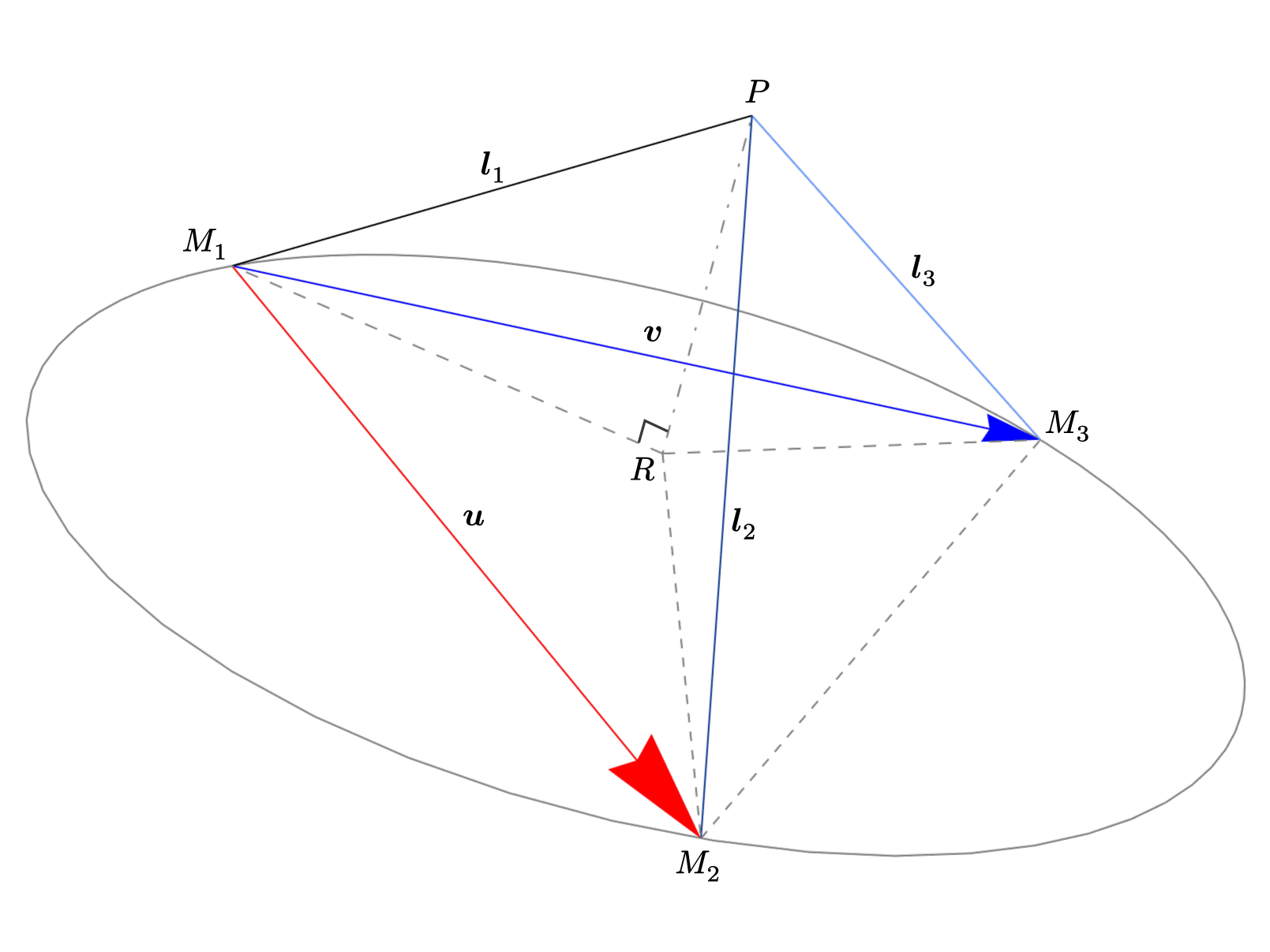
现在我们已经可以求出 \(M_i\) 的位置了. 为了进一步求出 \(\mathbf{l}_i\) 以得到 \(P\) 的位置, 注意到 \(l_i\) 都相等, 因此 \(\mathbf{l}_i\) 为圆锥 \(P-\odot{M_1 M_2 M_3}\) 的母线; \(P\) 为顶点. 圆锥的高 \(PR\) 垂直于底面; \(R\) 为三角形 \(M_1 M_2 M_3\) 的外心. 我们将要利用这一几何关系, 首先求出 \(R\) 的位置, 而后计算向量 \(\overrightarrow{RP}\), 进而得到所求点 \(P\).

三角形外心#

首先来解决求已知三角形外心位置的问题.

顶点信息包含在向量 \(\mathbf{u}\) 与 \(\mathbf{v}\) 中, 并且保证 \(\mathbf{u}\), \(\mathbf{v}\), \(\mathbf{n}\) 是按右手排列的, 即 \(\mathbf{n} = \mathbf{u} \times \mathbf{v}\), \(\mathbf{n}\) 为圆锥的高所在的方向. 可以找到 \(\{\mathbf{u}, \mathbf{v}\}\) 的一组对偶向量 \(\{\mathbf{u}_\perp, \mathbf{v}_\perp\}\) 满足 \(\mathbf{u} \cdot \mathbf{u}_\perp = \mathbf{u}^T \mathbf{u}_\perp = 0\), \(\mathbf{v} \cdot \mathbf{v}_\perp = 0\), 只需令 \(\mathbf{u}_\perp = \mathbf{u} \times \hat{\mathbf{n}}\), \(\mathbf{v}_\perp = \mathbf{v} \times \hat{\mathbf{n}}\).

此时 \(\{\mathbf{u}, \mathbf{u}_\perp\}\) 与 \(\{\mathbf{v}, \mathbf{v}_\perp\}\) 分别构成平面的基, 可以将外心坐标 \(\mathbf{r}\) 写为 \(\mathbf{r} = \frac{1}{2} \mathbf{u} + \lambda \mathbf{u}_\perp = \frac{1}{2} \mathbf{v} + \mu \mathbf{v}_\perp\), 移项得 \(\frac{1}{2} (\mathbf{u} - \mathbf{v}) = \mu \mathbf{v}_\perp - \lambda \mathbf{u}_\perp = (\mathbf{u}_\perp, \mathbf{v}_\perp) (-\lambda, \mu)^T\). 令 \(A := (\mathbf{u}_\perp, \mathbf{v}_\perp)\), 有方程

因为 \(\mathbf{u}\) 与 \(\mathbf{v}\) 都是三维矢量, 这个方程是超定的, 但是我们可以转换为最小二乘问题

这就变成了适定方程, 可以求解.

注意到 \(\|\mathbf{u}_\perp\| = \|\mathbf{u}\|\), 因为 \(\mathbf{u}\) 与 \(\hat{\mathbf{n}}\) 是正交的; \(\mathbf{u}^T A = (\mathbf{u}^T \mathbf{u}_\perp, \mathbf{u}^T \mathbf{v}_\perp) = (0, \mathbf{u} \cdot (\mathbf{v} \times \hat{\mathbf{n}})) = (0, n)\); \(\mathbf{v}^T A = (-n, 0)\), 可得

方程改写为

其中 \(S\) 为三角形面积 \(S := \frac{1}{2} \|\mathbf{u} \times \mathbf{v}\| = \frac{1}{2} n\).

使用克莱姆法则求解 \(\lambda\), 有

即

将这一结果代入 \(\mathbf{r}\) 的表达式中, 可得

圆锥顶点#

\(R\) 点的坐标利用上面的公式可以写为

其中 \(\mathbf{r}(\mathbf{u}, \mathbf{v}) = \mathbf{r}\).

此时 \(RP\) 的长 \(h\) 也容易求出, \(h = \sqrt{l^2 - r^2}\), 则 \(\overrightarrow{RP} = h \, \hat{\mathbf{n}}\).

至此已完成正向运动学建模.

代码#

import numpy as np
from numpy.linalg import norm


gg = 1.
LL = 1.
ll = 2.

def g_(phi):
    """从原点 O 到底盘上关节固定点 B 的向量: g"""
    i = np.array([1.,0,0])
    j = np.array([0,1.,0])
    return gg*(i*np.cos(phi) + j*np.sin(phi))

def L_(g: np.ndarray, theta):
    """从 B 到传动机构中途点 M 的向量: L"""
    k = np.array([0,0,1.])
    return LL*((g/norm(g))*np.cos(theta) + k*np.sin(theta))

def l_(u: np.ndarray, v: np.ndarray):
    """从 M 到目标点 P 的向量: l"""
    uu2 = norm(u)**2
    vv2 = norm(v)**2
    n   = np.cross(u, v)
    SS  = norm(n) / 2
    r   = (uu2*vv2*(u+v) - (u@v)*(vv2*u+uu2*v)) / (8*SS**2)
    rr2 = norm(r)**2
    nn  = np.sqrt(ll**2 - rr2)
    n   = (n / norm(n)) * nn
    return r + n


def fk(thetas: np.ndarray):
    """正运动学

    根据广义坐标: 极角 theta_i 求解终端位置 P,
    theta 按右手顺序排列."""
    phis = 2*np.pi/3*np.array([0.,1.,2.])
    O = np.zeros(3)
    M_s = np.zeros((3,3))
    for i, (phi, theta) in enumerate(zip(phis, thetas)):
        g = g_(phi)
        B = O + g
        L = L_(g, theta)
        M = B + L
        M_s[i] = M
    l = l_(M_s[1]-M_s[0], M_s[2]-M_s[0])
    P = M_s[0] + l
    return P

反向运动学#

普通机器人的逆运动学解算总是比正运动学困难得多, 但 Delta 机器人恰恰是个例外. 反向运动学, 或逆运动学的任务是已知末端 \(P\) 的位置, 求解广义坐标, 也就是极角 \(\theta_i\).

令 \(\mathbf{a} := \overrightarrow{BP} = P - \mathbf{g}\), 显然 \(\mathbf{a} - \mathbf{L} = \mathbf{l}\). 两边平方得 \(L^2 + a^2 - 2 \; \mathbf{L} \cdot \mathbf{a} = l^2\). 又因为 \(\mathbf{L} = L (\hat{\mathbf{k}} \sin{\theta} + \hat{\mathbf{g}} \cos{\theta})\), 有

令 \(A = 2L \, \mathbf{a} \cdot \hat{\mathbf{k}}\), \(B = 2L \, \mathbf{a} \cdot \hat{\mathbf{g}}\), \(C = l^2 - L^2 -a^2\), 线性三角方程 \(A \sin{\theta} + B \cos{\theta} + C = 0\) 的解即为所求.

线性三角方程#

形如 \(A \sin{x} + B \cos{x} + C = 0\) 的方程称为线性三角方程 (Linear Trigonometric Equation). 求解它的方法有以下几种:

恒等变换#

利用恒等变换 \(A \sin{x} + B \cos{x} = R \sin{(x + \phi)}\), 其中 \(R = \sqrt{A^2+B^2}\), \(\cos{\phi} = \frac{A}{R}\), \(\sin{\phi} = \frac{B}{R}\).

于是原方程变成 \(R \sin{(x+\phi)} + C = 0\), 即 \(\sin{(x+\phi)} = -\frac{C}{R}\). 设 \(\alpha = \arcsin{(-\frac{C}{R})}\), 则解为 \(x + \phi = \alpha\) 或 \(x + \phi = \pi - \alpha\). 所以, 在一个周期内, \(x = -\varphi + \alpha\) 或 \(x = -\varphi + \pi - \alpha\).

正切半角#

做换元 \(t := \tan\frac{x}{2}\), \(\sin x = \frac{2t}{1+t^2}\), \(\cos x = \frac{1-t^2}{1+t^2}\). 原方程化为二次方程 \((A - C) \; t^2 + 2B \; t + (A + C) = 0\). \(t\) 很容易解出, 为 \(t = \frac{-B \pm \sqrt{B^2+C^2-A^2}}{A-C}\); 再由 \(x = 2\arctan t\) 得解.

代码#

import numpy as np
from numpy.linalg import norm


gg = 1.
LL = 1.
ll = 2.

def solve_lte(A, B, C):
    """解线性三角方程 (Linear Trigonometric Equation)
    `A sin(x) + B cos(x) + C = 0`

    当无解 (解不为实数) 时抛出一个 `ComplexWarning` 异常"""
    delta = A**2 + B**2 - C**2
    if delta < 0:
        raise np.exceptions.ComplexWarning
    # 另一个解:
    # np.arctan2(-A*C + np.sign(A)*B*np.sqrt(delta), -B*C - np.sign(A)*A*np.sqrt(delta))
    return np.arctan2(-np.sign(A)*A*C - B*np.sqrt(delta), -np.sign(A)*B*C + A*np.sqrt(delta))


def ik(P: np.ndarray, phi):
    """逆运动学

    找到目标点移动到指定位置 P 时, 方位角为 phi 的一支应该具有的极角 theta.
    """
    g  = g_(phi)
    k  = np.array([0,0,1.])
    a  = P - g
    aa = norm(a)
    if aa > ll + LL:
        raise ValueError(P)
    g_h = g/gg
    return solve_lte(2*LL*(a@k), 2*LL*(a@g_h), ll**2-aa**2-LL**2)

动力学#

动力学的中心问题在于求出雅可比矩阵, 它可以建立广义速度与末端速度的关系, 进一步可以得出力矩到末端力的映射. 结合上面运动学建模, 可以获取我们关系的末端全部信息, 包括力, 位置与速度.

令末端 \(P\) 的位置为 \(\mathbf{p}\), 广义坐标 \(\mathbf{\theta} = (\theta_1, \theta_2, \theta_3)^T\), 所需的雅可比矩阵为 \(J = \frac{\partial \mathbf{p}}{\partial \mathbf{\theta}}\), 即

也即

其中 \(\mathbf{v}\) 表示末端速度, \(\dot{\mathbf{\theta}}\) 表示对 \(\mathbf{\theta}\) 求导.

对于我们讨论的非冗余 Delta 机构, 其末端自由度与广义坐标维度相等, 这意味着在非退化位形下 \(J\) 满秩. 因此, 任意满足 \(\dot{\mathbf{\theta}} \rightarrow \mathbf{v}\) 的线性映射都唯一是 \(J\), 我们只需找到速度是如何从起始端传递到末端即可求出 \(J\). 对于这种末端位置高度非形式化的机构, 求微分非常复杂, 几乎不可能求出, 上面的讨论给出了另一种求解 \(J\) 的方式. 回到我们关心的 Delta 机器人, 只需做速度分解即可.

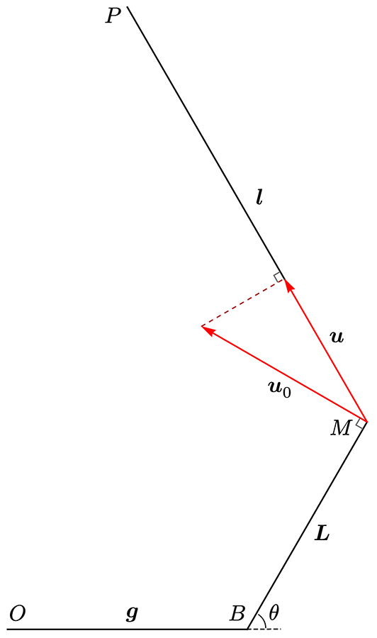
主动臂 \(BM\) 转动在 \(M\) 点产生的速度为 \(\mathbf{u}_0\), 令 \(\theta\) 的正方向为右手方向 (指向纸面之外), 则

其中 \(\mathbf{\omega} = \dot{\theta} \, (\mathbf{g} \times \mathbf{L})^\wedge\), \((\cdot)^\wedge\) 表示归一化.

进一步, 通过从动杆 \(MP\) 传递到末端的速度为 \(\mathbf{u}\), 它是 \(\mathbf{u}_0\) 在 \(\mathbf{l}\) 上的投影, 即

即

其中 \(\hat{\mathbf{L}}_\perp := \hat{\mathbf{k}} \cos\theta - \hat{\mathbf{g}} \sin\theta\).

三个从动杆上的速度在非退化位形下是线性无关的, 于是它们构成末端速度空间的一组基 \(\{\mathbf{u}_i\}\), 每个 \(\mathbf{v}\) 都是它们的线性组合, 即有

令 \(\mathbf{J} := L \, (\hat{\mathbf{l}} \cdot \hat{\mathbf{L}}_\perp) \, \hat{\mathbf{l}}\), 且同样 \(\hat{\mathbf{L}}_\perp = \hat{\mathbf{k}} \cos\theta - \hat{\mathbf{g}} \sin\theta\), 则

在实际应用中, 一般已知 \(\mathbf{\theta}\) 与 \(\mathbf{p}\), 要求 \(J\). 此时只需使用很小的开销计算 \(\mathbf{L}\) 和 \(\mathbf{L}_\perp\), 而后求出 \(\mathbf{l} = \mathbf{p} - \mathbf{L} - \mathbf{g}\), 就可应用公式. \(\mathbf{g}\) 和 \(\hat{\mathbf{k}}\) 应当是缓存的. 上述提到的向量长度都已知, 因此归一化的开销同样很小.

增量更新#

考虑一个运动的 Delta 机器人, 我们知道它当前时刻的 \(\mathbf{\theta}\) 和 \(\mathbf{p}\), 以及 \(J\) 和很短时间内广义坐标的改变 \(\mathrm{d} \mathbf{\theta}\), 此时末端位置的改变也很容易求出 \(\mathrm{d} \mathbf{p} = J \, \mathbf{d} \mathbf{\theta}\). 如何求解 \(\mathrm{d} t\) 时间后的雅可比 \(J'\)? 显然, 从头求解一遍运动学是不划算的, 这一操作过于昂贵, 而且上面的信息已经足够我们求解 \(J'\). 此时更好的方法是求出 \(\mathrm{d} J\), 而后由 \(J' = J + \mathrm{d} J\) 得出 \(J'\), 这被称为增量更新.

已知 \(\mathrm{d} \mathbf{L}\) 和 \(\mathrm{d} \mathbf{p}\), 那么 \(\mathrm{d} \mathbf{l} = \mathrm{d} \mathbf{p} - \mathrm{d} \mathbf{L}\), 并且 \(\mathrm{d} \mathbf{L} = L \, \mathrm{d}\theta \, \hat{\mathbf{L}}_\perp\), \(\mathrm{d} \hat{\mathbf{L}}_\perp = -\hat{\mathbf{L}} \, \mathrm{d} \theta\). 对于 \(J\) 的分量 \(\mathbf{J}\), 有

这三项的计算都比较廉价.

计算出 \(\mathrm{d} \mathbf{J}\) 后, 就有

如此一来便可计算 \(J' = J + \mathrm{d} J\).